
The symmetry beneath it all
Part 7 of "The Inference Universe": Why the laws of physics look like inference, and what's actually real


In 1959, two physicists proposed an experiment that shouldn’t work.
Yakir Aharonov and David Bohm predicted that an electron could be affected by a magnetic field it never touches. Send an electron around a solenoid - a coil with a magnetic field confined entirely inside it. The electron travels only through regions where the magnetic field is exactly zero. Yet its behavior changes depending on the field inside the coil.
This was heresy. In classical physics of the time, fields are what’s real. The magnetic field B exerts forces. The magnetic potential A is just a mathematical convenience; a bookkeeping device. Where B is zero, nothing physical should happen. Potential, to physicist of the time; was a mathematical instrument, not a physical reality.
But the experiment was done. Aharonov and Bohm were right. The electron’s quantum phase shifts based on the potential A, even where the field B vanishes.
Something the smartest of us ever thought was “just mathematics” turned out to be physically real. And the thing we thought was fundamental - the local field; turned out to be secondary to this potential.
This is where our inference frame faces its deepest test. We’ve claimed the universe is an inference machine. Now we must ask: what exactly is being inferred? What’s real: fields, potentials, or something stranger still? And what does “local” even mean when quantum mechanics enters the picture?
Let’s find out.
The old-school hierarchy of reality
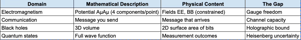
Start with what seems obvious. In physics, we have had an hierarchy for ages:
Level 1: Observables What you can measure. The magnetic field strength at a point. The electric force on a charge. The position of a particle. These are “real” in the most operational sense; you can build instruments to detect them.
Level 2: Fields The are things that determine the above observables. The electric field E, the magnetic field B. You can’t see a field directly, but you can see its effects everywhere. Fields seem pretty real, coz the observables experience the field’s effects.
Level 3: Potentials The things that determine the fields. The electric potential φ, the magnetic vector potential A. The fields are derivatives of the potentials:
E = -∇φ - ∂A/∂t
B = ∇ × A
Potentials seem like mathematical conveniences. They were created for mathematical ease. You can change them with (gauge transformation) without changing the fields. So they can’t be “real”; different potentials give the same physics.
Level 4: Phases The quantum mechanical phase that accumulates as a particle moves. The phase depends on the potential integrated along the path. But absolute phase is unobservable; only the phase differences really matter.
The classical intuition says: reality flows downward. Phases determine potentials, potentials determine fields, fields determine observables. The higher levels are “just math” for the sake of calculation ease.
The Aharonov-Bohm effect inverts this. The potential, supposedly just math; has real world, physical effects that the field doesn’t capture. The hierarchy that had been assumed for ages to be true, is wrong, or at least incomplete.
Locality: the classical physics story
Classical physics is local. This is one of it’s deepest assumptions and most crucial one.
Locality: What happens at a point depends only on conditions at that point and its immediate neighborhood.
Fields are the machinery of that locality. Instead of action at a distance (Newton’s gravity reaching across empty space), here we have fields that exist everywhere and propagate at a finite speed.
The electric field at point P determines the force on a charge at P. The charge doesn’t need to “know” about distant sources; it only needs to know the local field value and behaves accordingly.
The inference translation
In the inference frame, locality means:
Local inference: The update at each point depends only on local data (field values) and local priors (how this point relates to neighbors).
This is like a cellular automaton. Each cell updates based on its neighbors. The global pattern emerges from these local rules.
Similarly, fields are the channels for local inference. The field value at P is the “message” available at P. The laws of physics are the local update rules.
This is clean. This is elegant. This is also wrong; or at least incomplete.
The Aharonov-bohm effect: when path matters
Here’s the setup. An electron source emits electrons toward a screen. Between source and screen is an impenetrable solenoid; a thin coil with magnetic field B confined entirely inside. The electron can pass on either side but cannot enter the solenoid.
Outside the solenoid, B = 0 everywhere. The magnetic field vanishes in the entire region the electron can access. By the locality principle, the electron shouldn’t “know” about the field inside.
But quantum mechanics says the electron’s phase accumulates according to:
φ = (e/ℏ) ∮ A · dl
Mathematically, this is described as: the phase depends on the line integral of the potential A around the path; even where B = 0.
When electrons going around different sides of the solenoid meet at the screen, their phases differ. This phase difference produces interference fringes. Change the current in the solenoid (changing B inside, changing A outside), and the fringes shift.
The electron is affected by a field it never encounters. And this is crazy.
What this means
Option 1: Potentials are real. The potential A, not just the field B, has physical meaning. The electron couples to A directly. Gauge transformations change something physically real.
Problem: Gauge transformations are supposed to be unphysical; different mathematical descriptions of the same physics. If A is real, why/how can we change it arbitrarily?
Option 2: The phase is real. What’s physical isn’t A itself, but the integral ∮ A · dl around a closed loop. This is gauge-invariant; meaning it doesn’t change under gauge transformations. The “reality” lives in the path, not the point.
Option 3: Non-locality is real. The electron’s state depends on global information (the flux through the solenoid), not just local information (the field at its location). Locality fails; but in a very subtle way.
The inference translation
In inference terms, the Aharonov-Bohm effect says:
Your posterior depends on the path you took, not just where you are now.
The accumulated phase is like accumulated evidence. Two observers who end up at the same point, but arrived via different paths, have different posteriors; even if the local “data” (field) is identical. This is not standard Bayesian inference, where only the current data and prior matter. This is path-dependent inference - the history of the thing or entity is baked into the state of the entity.
The potential A encodes “how inference accumulates along paths.” The field B = ∇ × A encodes “the local rate of accumulation.” But the total accumulation can be non-zero even when the local rate is zero everywhere along the path; if the path encloses a region where things are different.
This is non-locality, but of a specific kind, mathematically termed as: topological non-locality. The electron doesn’t interact with the solenoid directly. But its path topology, whether it goes around the solenoid or not; seems to matter.
Gauge symmetry: what can you actually infer?
Let’s dig into gauge invariance, because it’s the key to understanding what’s real. There’s a bit of high-school+ maths here.
A gauge transformation changes the potential:
A → A + ∇χ
φ → φ - ∂χ/∂t
where χ is any smooth function. This changes A and φ, but leaves the fields E and B unchanged. It also leaves the Aharonov-Bohm phase ∮ A · dl unchanged (because the added term ∮ ∇χ · dl = 0 for a closed loop).
What gauge invariance means
Gauge invariance says: certain aspects of the mathematical description are not physically meaningful. Eg., The absolute value of the potential at a point is meaningless. Only potential differences matter (for φ) or circulationsmatter (for A).
This is exactly like coordinate invariance. The absolute position (x, y, z) = (3, 4, 5) is meaningless; it depends on where you put the origin. Only relative positions really matter.
The inference translation
Gauge symmetry means certain degrees of freedom are unobservable; they don’t enter the likelihood function.
You can never design an experiment that measures the absolute potential. No data will ever distinguish A from A + ∇χ. So inference about the absolute potential is impossible; the posterior equals the prior, always.
Gauge-invariant quantities are what you can infer with measurement:
Field strengths (E, B)
Phase differences
Topological invariants (like total flux)
The gauge potential A is like a “latent variable” that you marginalise over. It’s useful for mathematical calculations, but the physical content lives in the invariants.
Why gauge theories?
Here’s a deep question: why does physics use gauge theories at all, if the gauge freedom is unphysical?
The answer: theory and locality requires it.
You want a theory where interactions are local; a charge at point P interacts with the field at point P. But you also want the theory to respect certain global symmetries (like the phase symmetry of quantum mechanics).
The price of combining locality with global symmetry is via gauge freedom. You get extra mathematical degrees of freedom that encode “how to connect local descriptions consistently.”
The gauge potential A is called a connection in differential geometry. It tells you how to compare phases at different points. It tells you how to “parallel transport” the quantum state from one location to another.
This is an inference machinery: the gauge potential is the grammar that lets local inferences combine into global consistency.
Quantum phase as an accumulated prior
Let’s make the inference interpretation precise.
In quantum mechanics, the state of a particle is described by a wave function :
ψ(x) = |ψ(x)| e^(iθ(x))
The magnitude |ψ|² gives probabilities. The phase θ determines interference.
As a particle moves through space, its phase accumulates:
θ(path) = ∫_path (p · dx - E dt) / ℏ
where p is momentum and E is energy. In the presence of electromagnetic fields, this becomes:
θ(path) = ∫_path [(p - eA) · dx - (E - eφ) dt] / ℏ
The potentials A and φ modify how phase accumulates.
The inference translation of this
Quantum phase is the log-probability accumulated along a path.
More precisely, in the path integral formulation:
Amplitude = ∫ [all paths] exp(iS[path]/ℏ)
where S[path] is the action for that path.
Each path contributes with a weight e^(iS/ℏ). Paths with similar actions interfere constructively; paths with different actions interfere destructively.
The classical path (least action) is where the phase is stationary; all nearby paths have similar phases, so they add up. This is why classical behavior emerges: the classical path dominates the sum.
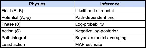
In Bayesian terms:
Each path is a hypothesis
The action S is (something like) the negative log-prior
The path integral is model averaging
The stationary phase approximation is the MAP estimate
The potential A modifies the action, and therefore modifies which paths contribute. The Aharonov-Bohm effect is: the potential changes the weights in the model average, even where the “local data” (field) is zero.
Bell’s theorem: when inferences can’t be local
Now we go further. The Aharonov-Bohm effect shows topological non-locality; that path dependence matters.
But quantum mechanics has a deeper non-locality: entanglement.
The setup
Two particles are prepared in an entangled state; say, with total spin zero. They fly apart to distant locations where Alice and Bob measure them.
Quantum mechanics predicts: the results will be correlated in a specific way. If Alice measures spin-up along some axis, Bob will measure spin-down along the same axis, with certainty.
This isn’t surprising by itself. Classical correlations can do this: if I put one red ball and one blue ball in two boxes, shuffle, and send them to Alice and Bob, their results will be correlated.
Bell’s Inequality
John Bell proved something shocking: the quantum correlations are stronger than any classical explanation allows.
If you assume:
Realism: Each particle has definite properties before measurement
Locality: Alice’s measurement doesn’t affect Bob’s particle (or vice versa)
Then you can prove an inequality that the correlations must satisfy.
Quantum mechanics violates this inequality. Experiments have confirmed the violation repeatedly. Hence one of the earlier assumptions must be wrong.
The inference translation of this
Bell’s theorem says: you cannot explain quantum correlations with local, independent priors.
If each particle had a “local hidden variable” λ , that provides a complete description of its state that determines all measurement outcomes; then the correlations would satisfy Bell’s inequality.
The violation means: the quantum state is not a product of local states. It’s irreducibly joint. Your high school probability basics do not work here.
Entanglement means the prior is over joint states, not products of local states.
You cannot write:
P(A, B) = ∫ P(A|λ) P(B|λ) P(λ) dλ
where A is Alice’s outcome and B is Bob’s. No assignment of local probabilities works. The correlation is fundamental, not derived from local properties.
What kind of non-locality are we talking about?
The type that doesn’t allow faster-than-light signaling. Alice can’t control her outcome, so she can’t send information to Bob through the correlations. The non-locality is in the correlations, not in any causal influence.
In inference terms:
Some inferences are irreducibly about relationships, not about the things themselves.
The entangled state doesn’t say “particle A has property X and particle B has property Y.” It says “the relationship between A’s outcome and B’s outcome is Z.” The relationship is primary; the individual properties are derived (upon measurement).
This is strange. But it’s consistent with our inference frame; if we proceed to accept that some priors are over joint configurations, not product distributions over local states.
Holography: when the boundary knows everything
Here’s perhaps the strangest result in modern physics. The holographic principle (from string theory and black hole physics) suggests:
The information content of a region of space is encoded on its boundary, not in its volume.
A black hole’s entropy (a measure of information content) is proportional to its surface area, not its volume. This is bizarre; you’d expect a bigger volume to hold more information.
The AdS/CFT correspondence goes further: a theory of quantum gravity in a volume is exactly equivalent to a theory without gravity on the boundary. The bulk and boundary are dual descriptions of the same physics.
The inference translation
Local inference in the bulk is equivalent to global inference on the boundary.
What happens “inside” (the volume) can be completely reconstructed from what happens “outside” (the boundary). What this translates to is that interior and exterior of a black hole are not independent; they’re related by a kind of inferential duality.
This is the ultimate limit of non-locality: there is no purely local information. Everything local is encoded globally, and vice versa.
For our inference frame, this suggests:
The universe’s inference is not localized in space. Spatial locality is an emergent, approximate description of a fundamentally non-local structure.
This is fully speculative. But for me it aligns with something we’ve seen throughout: the “local” description (fields at a point) is always embedded in global structure (gauge invariance, topological effects, entanglement).
Symmetry breaking: when priors collapse
We’ve talked about symmetry as invariance, of transformations that don’t change the physics. Now let’s talk about what happens when symmetry breaks.
The Mexican hat
Consider a potential shaped like a Mexican hat (sombrero):
V(φ) = -μ²|φ|² + λ|φ|⁴
This potential has a circular symmetry. You can rotate φ in the complex plane and the potential doesn’t change.
But the minimum of the potential isn’t at φ = 0. It’s on a circle |φ| = v. The system has to “choose” a point on that circle; and any choice breaks the rotational symmetry.
The laws are symmetric. But the ground state is not. This is spontaneous symmetry breaking.
The inference translation
Symmetry breaking is what happens when the prior is symmetric but the posterior is not symmetric.
The potential is like a symmetric prior; no direction is favored. But the system must settle into a definite state (the posterior). That state necessarily picks a direction.
This is like a Bayesian model with a symmetric prior that gets “broken” by data. The prior says “all directions equally likely.” The data (or thermal fluctuations, or quantum fluctuations) forces a choice.
Why Symmetry Breaking Matters
Symmetry breaking generates:
Mass: The Higgs mechanism gives particles mass through symmetry breaking
Phase transitions: Water freezing, magnets magnetizing, superconductivity
Diversity: Why the universe isn’t a uniform soup
In inference terms: symmetry breaking is how the universe computes definite outcomes from symmetric rules.
The laws are symmetric (the prior is flat). But actual states are specific (the posterior is peaked). The dynamics of inference - thermal fluctuations, quantum measurement, cosmic expansion; drive the system toward symmetry-broken states.
The synthesis: what’s actually real?
Let’s pull this together. We started with a hierarchy: observables → fields → potentials → phases. We asked what’s “real.”
Here’s what we’ve learned:
1. Fields are not the whole story. The Aharonov-Bohm effect shows that potentials, or rather, their topological invariants; have physical effects that fields don’t capture.
2. Locality is subtle. Classical locality (each point depends only on neighbors) works for fields. But quantum effects show path-dependence (Aharonov-Bohm) and irreducible correlations (entanglement) that aren’t local in the classical sense.
3. Gauge invariance tells us what’s inferable. The gauge freedom isn’t a nuisance; it’s a feature. It tells us exactly what can and can’t be learned from data. Gauge-invariant quantities are what’s real in the epistemic sense.
4. The phase is the inference. Quantum phase accumulates along paths, encoding the “log-probability” of trajectories. The phase is how the universe keeps track of which paths contribute to the outcome.
5. Some inference is irreducibly global. Entanglement, holography, and topology all point to the same conclusion: you can’t always factor the world into independent local pieces. Some structure is fundamentally relational.
What’s real?
Here’s a proposal:
What’s “real” is what’s invariant under the transformations that don’t change predictions.
Gauge-invariant quantities are real (fields, phase differences, topological invariants)
Gauge-dependent quantities are not real (absolute potentials, absolute phases)
Relations can be more real than relata (entangled correlations, holographic duality)
This is an inferentialist criterion for reality: the real is what can be inferred from all possible data.
The lost bits: Gauge Freedom, Channel Capacity, and the Limits of physical information
There’s a question lurking beneath everything we’ve discussed: what’s the relationship between gauge freedom and Shannon’s channel capacity? Both seem to involve information that “isn’t there”; but in different ways.
Shannon’s Law says: given a channel with capacity C, you cannot reliably transmit more than C bits per second. Attempt to exceed this, and information is lost to noise.
Gauge invariance says: certain degrees of freedom in our mathematical description don’t correspond to physical observables. No experiment can ever measure them.
At first, these seem unrelated. Shannon’s lost bits were real information destroyed by noise. Gauge freedom is redundant description; bits that were never physical to begin with.
But when we look deeper, a pattern emerges.
The universal constraint
Both phenomena reflect a single principle:
The physical information content is less than the mathematical description suggests.
This shows up everywhere:
The pattern: reality encodes less information than our descriptions assume.
Gauge Freedom as untransmittable information
Consider what gauge invariance actually says. The potential AA at a point can be shifted:
A→A+∇χA→A+∇χ
for any smooth function χχ, without changing any physical prediction. The absolute value of A(x)A(x) at a single point is *unmeasurable in principle*.
In Shannon’s language: the gauge-dependent parts of AA are information that cannot be transmitted through any physical measurement channel. Not because of noise ; because they aren’t in the physical signal at all.
This is more severe than Shannon’s limit. Shannon says some bits can’t get through this channel given this noise level. Gauge invariance says some “bits” can’t get through any channel; they’re not physical degrees of freedom.
Gauge freedom = information that no measurement, however precise, can ever extract.
The Holographic connection
The relationship becomes precise when we consider the holographic bound. Let’s take a deep dive into the physics of it. The Bekenstein bound limits the maximum entropy (information) in a spherical region:
S_max = 2π k_B R E / ℏc
For a black hole, this becomes what’s known as the Bekenstein-Hawking entropy:
S = A / 4ℓ_P²
where A is the surface area and ℓ_P = √(ℏG/c³) is the Planck length (about 10⁻³⁵ meters).
This is a channel capacity for spacetime itself:
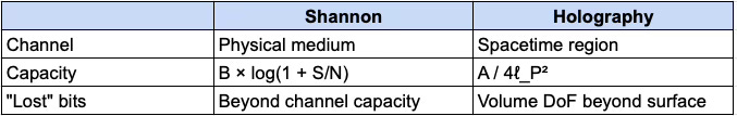
The holographic principle says the bulk in a volume is gauge-equivalent to the boundary. The apparent “extra” degrees of freedom in the volume aren’t independent; they’re redundantly encoded on the surface.
The volume bits therefore aren’t lost to noise. They were never independent information to begin with. Just like gauge freedom.
Redundancy as the price of locality
Here’s perhaps the deepest connection. In Signal processing or Comp Sci, when you encounter error-correcting codes, you encode k bits of message into n bits of transmission (n > k). The extra n − k bits are redundancy; they carry no new information but protect the message against noise.
In gauge theory, you describe physics with more variables than physical degrees of freedom. The extra gauge freedom carries no physical information but makes the theory local and well-defined.
Why do we need gauge freedom at all? Because we want two things to be consistent simultaneously:
Local interactions: A charge at point P responds only to the field at P
Global symmetry: The physics respects phase invariance of quantum mechanics
The price of combining these is gauge freedom; extra mathematical structure that lets local descriptions combine into a globally consistent picture.
This is exactly analogous to Shannon’s coding theorem: to transmit reliably at capacity, you need redundancy. The redundancy isn’t waste; it’s what makes reliable transmission possible.
Gauge freedom is the error-correcting overhead that makes local physics possible.
The Potential as distributed code
If we think about it, the Aharonov-Bohm effect reveals the structure precisely. The local value A(x) at a point is gauge-dependent, it’s unphysical. But the integral around a closed loop:
Φ = ∮ A · dl
is gauge-invariant, real and physical. The magnetic flux through the enclosed area affects the electron’s phase, even where the field B = ∇ × A vanishes.
The information is there, but distributed. You can’t read it from any single point. You need the whole path.
This is exactly like holographic encoding:
Information is spread across the encoding
Local measurements don’t reveal the full content
You need non-local access (path integral, boundary measurement) to recover it
The “lost bits” aren’t lost at all. They were never meant to be read locally. The local values of A are the codeword, not the message. The message is in the global, gauge-invariant structure.
The unified picture
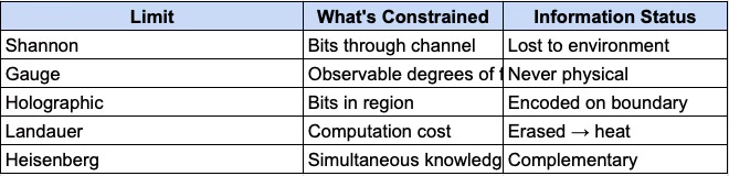
Let’s map these limits together:
The deeper unity
We’ve now seen three layers of connection between physics and inference:
Dynamics: Physical evolution follows variational principles identical to Bayesian updating
Observability: Gauge invariance determines what can be inferred from data
Capacity: Information limits (Shannon, holographic, Landauer) constrain how much inference is possible
Let’s unify these into a single picture. The physics-inference correspondence now extends beyond dynamics to include structural constraints:
DYNAMICS (how it moves):
OBSERVABILITY (what's real):
CAPACITY (how much):
The correspondence isn’t partial; it’s total. Every major structure in physics maps to an equivalent structure in inference.
The 3 constraints
Physical inference is bounded in three ways:
1. What can be inferred (Gauge)
Not everything in our mathematical description is physical. Gauge-invariant quantities such as fields, phase differences, topological invariants; are what measurement can access. The rest are coordinate artifacts.
Observable ⟺ Gauge-invariant ⟺ Inferable
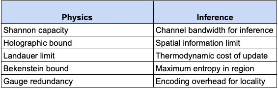
2. How much can be inferred (Capacity)
Even for physical quantities, there are limits.
Shannon’s theorem: C = B × log₂(1 + S/N)
The holographic bound: S_max = A / 4ℓ_P²
Landauer’s principle: E_min = k_B T × ln(2) per bit erased
These aren’t separate limits. They’re aspects of one constraint:
the universe has finite information-processing capacity.
3. How inference must be structured (Locality + Consistency)
We want local physics; interactions at a point depend only on fields at that point. We also want global consistency: the laws respect symmetries. The price of need both of these to be true, together; is gauge freedom: redundant degrees of freedom that encode “how to connect local descriptions.”
This is the same tradeoff as error-correcting codes: redundancy enables reliability. Gauge structures enable locality.
The variational core: at the mathematical center, one structure appears everywhere:
Minimize F = E_q[log q − log p]
This is:
Free energy in statistical mechanics
Variational free energy in Bayesian inference
Action in classical mechanics (via Legendre transform)
Relative entropy (KL divergence) in information theory
The universe continously extremizes this functional. So does optimal inference. They’re fundamentally the same operation.
In physics: δS = 0 implies equations of motion
Similarly, in inference: ∇F = 0 implies optimal posterior
The Euler-Lagrange equations are the conditions for optimal belief updating. Hamilton’s equations are the flow of probability through phase space. Quantum mechanics is inference over paths, weighted by exp(iS/ℏ).
Why these constraints?
Here’s the deep question: why does reality have these particular constraints?
The self-consistency hypothesis: The universe is an inference machine that must process its own states. For this to work:
Information must be finite, otherwise updates can’t complete
Information must be distributed, otherwise local processing is impossible
Redundancy must exist, otherwise errors propagate catastrophically
The constraints we observe such as gauge freedom, holographic bounds, channel capacity, they are are precisely what’s required for a self-consistent, locally-processable inference system. Therefore, gauge freedom isn’t a bug in our description. It’s the encoding structure that lets the universe compute locally while remaining globally coherent. The holographic bound isn’t a strange limit on black holes. It’s the statement that spatial regions are channels with finite capacity. Shannon’s theorem isn’t just about telephone wires anymore. It’s the universal constraint on any physical channel; including spacetime itself.
The information-theoretic reformulation
We can now state the unity precisely:
Physics is inference under three constraints:
Observability: Only gauge-invariant quantities are physically measurable
Capacity: Information flow is bounded by Shannon/holographic/Landauer limits
Locality: Inference must be locally computable, requiring gauge redundancy
The laws of physics: Maxwell’s equations, Einstein’s equations, the Standard Model; they are the unique (or nearly unique) solutions satisfying these constraints.
This inverts the usual view. We normally ask: “Given the laws, what happens?” The inference view asks: “Given the constraints on consistent inference, what laws are possible?”
The answer: approximately the laws we have. The universe isn’t arbitrary. It’s what consistent, finite, local inference looks like.
Symmetry as compression
One more connection to take note exists. Symmetries reduce the hypothesis space for inference; they tell you what doesn’t need to be inferred.
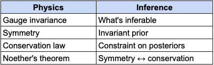
If your theory is rotationally symmetric, you don’t infer absolute orientation. If it’s time-translation symmetric, you don’t infer absolute time. The symmetry compresses the inference problem. Conservation laws are the consequence of this symmetry: energy, momentum, charge are conserved because the corresponding degrees of freedom are “factored out” of the inference.
Noether’s theorem, in inference terms can be put as:
Symmetry ⟺ Compressed prior ⟺ Conservation law
This is why symmetry is so powerful. It’s not just an aesthetic math. It’s computational; it reduces the information that must be processed.
The universe’s symmetries are its compression algorithm. The conservation laws therefore are the invariants under that compression. Together, they make possible propogation of finite inference over an apparently infinite world.
The Gauge-Holographic-Shannon triangle
Let’s see how the three information constraints relate:
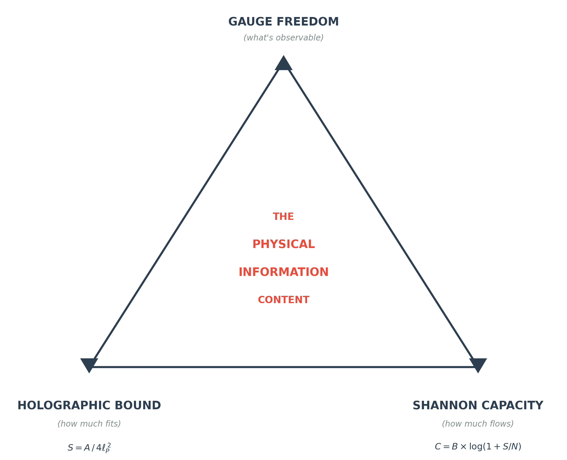
Gauge determines the type of information (what’s real)
Holographic determines the amount in a region (what fits)
Shannon determines the rate through a channel (what flows)
All three must be satisfied simultaneously. Physical information is therefore:
Gauge-invariant (observable in principle)
Holographically bounded (fits in the region)
Shannon-limited (transmittable through the channel)
The intersection is small. Most “information” in our mathematical descriptions fails one or more constraints. What survives reality is eventually what we see and measure as physics.
The emergence of spacetime
Here’s a personal, speculative extension to all the theory build up. If gauge freedom is encoding structure, and holographic bounds relate bulk to boundary, then perhaps spacetime itself is emergent; it’s the structure that encodes more fundamental quantum information.
The AdS/CFT correspondence suggests exactly this: a gravitational theory in the bulk is equivalent to a non-gravitational theory on the boundary.
Therefore, the extra dimension is... what? Perhaps it’s the encoding depth: how much redundancy is built into the representation.
In this view:
Spacetime = encoding structure for quantum information
Gravity = the dynamics of that encoding
Gauge freedom = the redundancy that makes encoding robust
Holographic bound = the capacity of the code
We don’t have physics happening in spacetime. We have spacetime emerging from the structure and limitations of physical information.
Again, this is speculative. But it’s where the inference frame I currently have in my world model, pushed to its limit, seems to point at.
What this means
If this picture is right, what follows?
for Physics
I have always felt that physics isn’t just about predicting; it’s about the structure of prediction. Today, I feel the laws of physics aren’t arbitrary; they’re constrained by consistency requirements on inference:
Locality (local inference should be possible)
Symmetry (some things shouldn’t need inferring)
Gauge invariance (don’t count unobservables)
Unitarity (probabilities sum to one)
The specific laws we have (Standard Model, General Relativity) are the simplest consistent solutions to these constraints. What we term as “Physics” seems to be inference under constraints. Finding new physics therefore means finding what else the “consistency” requires.
for Philosophy
The debate between realism and anti-realism gets reframed. It’s not “is there a reality independent of observation?” but “what aspects of the mathematical description correspond to inferable structure?”
Gauge-invariant quantities are real in the sense that matters; they’re what any observer could learn. The rest is “coordinate” driven choices; they are just description, not the reality itself.
for AI & Intelligence
If the universe computes via variational inference, then intelligence; be it biological or silicon: is more of the same. Brains minimize free energy. AI minimizes loss functions. Both are running inference. The constraints that bind physics (finite information, local processing, redundant encoding) may also bind intelligence.
The difference between physics and thought isn’t the mechanism. It’s the complexity of the model and the nature of the data. A rock “infers” its trajectory. A brain infers the intentions of other agents. Same math, but vastly different sophistication.
for Meaning
Meaning, we said in Part 4, is computed relevance. Now we can add:
Meaning is what remains invariant under the transformations that don’t matter to you.
Your identity is what’s “gauge-invariant” about you; what remains stable across superficial changes. Your values are symmetries: transformations under which your preferences don’t change.
Finding meaning is finding invariants. Losing meaning is losing them.
We're not separate from this process of inference. Your and my brain runs variational inference. Your beliefs are posteriors. Our actions minimize expected free energy. You and I are the universe's inference, turned inward, modelling itself.
Coda: the symmetry beneath
Let me end with an mental image.
Beneath the phenomena - the particles, the fields, the forces; lies a deeper structure. It’s made of symmetries: transformations that leave the likelihood unchanged, degrees of freedom that can’t be inferred, constraints that shape what’s possible. The laws of physics aren’t commands imposed from “outside”. They’re the logical structure of consistent inference.
Meaning: Charge is conserved because the equations are symmetric under phase rotations. Energy is conserved because the equations don’t depend on when you start the clock. Momentum is conserved because space doesn’t have a preferred origin point where all the axis(s) meet.
The universe isn’t following rules. It’s embodying consistency.
And here’s the strange, beautiful thing: you and me are part of this. Your mind runs inference on the same principles. Your brain minimizes free energy, finds invariants, breaks symmetries to reach decisions.
When you understand something, really understand it; you’ve found the symmetry. The pattern that remains when details vary. The structure that’s robust to perturbation. The invariant.
When you act well wisely, in accordance with your values; you’re preserving your symmetries. Staying consistent with what you care about, even as circumstances change.
The universe is an inference machine. You’re a piece of it that got complex enough to notice.
Noticing is a kind of privilege. Use it. The symmetry beneath is what makes the chaos coherent. Finding it, in physics, in societies, in our own life; that’s the work.
This concludes “The Inference Universe” series.
Appendix: Key References
Y. Aharonov & D. Bohm : “Significance of Electromagnetic Potentials in the Quantum Theory” (1959). The original Aharonov-Bohm paper.
J.S. Bell : “On the Einstein Podolsky Rosen Paradox” (1964). The original Bell inequality paper.
Emmy Noether : “Invariante Variationsprobleme” (1918). The proof that symmetries yield conservation laws.
Richard Feynman : “Space-Time Approach to Non-Relativistic Quantum Mechanics” (1948). The path integral formulation.
C.N. Yang & R.L. Mills :“Conservation of Isotopic Spin and Isotopic Gauge Invariance” (1954). Foundation of non-Abelian gauge theory.
Juan Maldacena : “The Large N Limit of Superconformal Field Theories and Supergravity” (1998). The AdS/CFT correspondence.
Gerard ‘t Hooft :“Dimensional Reduction in Quantum Gravity” (1993). Early holographic principle ideas.
Chris Fuchs : “QBism, the Perimeter of Quantum Bayesianism” (2010). Quantum mechanics as Bayesian inference.
E.T. Jaynes : “Probability Theory: The Logic of Science” (2003). The deepest treatment of probability as inference.
Michael Nielsen & Isaac Chuang : “Quantum Computation and Quantum Information” (2000). Standard reference on quantum information.